Kyle Donnelly, Algorithmic Trader & Market Technician
July 12, 2026 · 16 min read
Backtesting trading: why paper profits fail in real execution
A strategy I tested last month printed a 2.1 Sharpe in-sample, 18% annualized return, and a maximum drawdown under 7%. Nice equity curve. Smooth enough to sell to someone who does not ask how fills work.
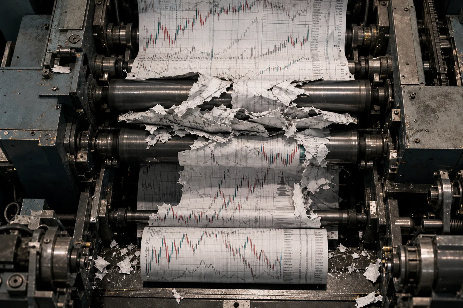
The Sharpe dropped below 0.8. The drawdown doubled. The edge did not disappear. The fantasy did.
That is the core problem with backtesting trading strategies. Most failures are not mysterious. They are mechanical. The model assumes prices you could not have traded, liquidity you could not have accessed, information you did not yet have, and regime stability the market never promised. A backtest is not a profit forecast. It is a debugging environment. Treat it as anything else and the market will invoice you for the difference.
The clean backtest is usually the dirty one
The first warning sign is not a bad backtest. It is a perfect one.
Straight-line equity curves, tiny drawdowns, high trade counts, and surgical entries usually mean the model has been allowed to cheat somewhere. Not always intentionally. Most algorithmic backtesting errors are boring. A timestamp is aligned incorrectly. A signal uses a closing price before the close exists. A universe includes only surviving stocks. A spread is assumed to be zero because the CSV only has last trade prices.
The retail misconception is that historical data is “truth.” It is not. It is a compressed artifact of a market that had queues, failed fills, stale quotes, missing ticks, corporate actions, halted securities, changing spreads, and participants reacting to the same prints your model is now calmly consuming.
I use historical data because there is no alternative. But I do not trust it. I interrogate it.
A basic moving-average crossover on daily bars might look harmless. Fast average crosses above slow average, buy at the close, exit on reverse cross. But if the signal is calculated using that same closing price and the fill is also booked at that close, the test is already optimistic. At the moment the close is known, that price is gone. You either execute before the close with incomplete information, or after the close with a different fill assumption.
That single detail can turn an average strategy into a fake asset manager.
The same problem gets worse intraday. On a five-minute bar, using high, low, and close to decide whether an entry, stop, and target were all touched inside the same candle is not analysis. It is fiction unless the engine knows the sequence of ticks. Many engines guess. Some choose the most favorable path. That is not backtesting. That is curve decoration.
A backtest that fills every signal cleanly is not conservative. It is an unpaid marketing department for your own bias.
Historical backtesting limitations are not an argument against testing. They are an argument against lazy simulation. The test should make the model fight through the same frictions the live strategy will face.
Slippage is not a parameter. It is the market pushing back
Slippage is the difference between the expected trade price and the actual executed price. That definition sounds simple. The implementation is not.
Most novice backtests apply slippage as a fixed number: one tick, two basis points, half a spread, whatever makes the spreadsheet feel mature. That is better than zero. It is still crude.
Real slippage changes with:
- Volatility regime. A one-cent assumption on a calm large-cap session is not the same as one cent during CPI release volatility.
- Order type. Market orders pay immediacy. Limit orders risk non-fill. Stop orders often become market orders at the worst part of the local distribution.
- Trade size relative to liquidity. A 100-share fill and a 50,000-share fill are not the same trade with a bigger font.
- Time of day. Open and close behavior is structurally different from midday drift.
- Spread dynamics. The bid-ask spread is a variable cost, not a decorative quote field.
- Signal crowding. If the signal is obvious, other models may be trying to access the same liquidity at the same moment.
This is where backtesting vs live trading starts to diverge aggressively. A historical bar tells you where price traded. It does not tell you whether your order would have been filled there, how much size was available before you, or how the book would have responded to your own participation.
For high-frequency trading, the problem becomes brutal. A strategy that relies on small price movements can have its expected value erased by commissions, exchange fees, spread, and latency. Latency is measured in milliseconds or microseconds in serious execution environments. Retail infrastructure usually should not pretend to compete in that arena. Not because retail traders are intellectually inferior. Because physics, routing, colocation, queue position, and fee tiers are not motivational variables.
Here is the version of cost modeling I prefer for early research. It is not perfect. It is honest enough to kill weak ideas quickly.
| Cost component | Naive backtest assumption | More realistic treatment |
|---|---|---|
| Commission | Often ignored | Applied per share, per contract, or per notional depending on venue and broker |
| Bid-ask spread | Zero or fixed | Variable by asset, time of day, and volatility regime |
| Slippage | One constant value | Scaled by spread, volatility, and order size relative to volume |
| Market impact | Ignored | Penalized when participation rate rises or liquidity is thin |
| Latency | Instant execution | Signal-to-order delay, next-bar execution, or timestamp-based simulation |
| Non-fills | Every limit order fills | Fill probability modeled from price path and queue assumptions |
The point is not to build a perfect market simulator. You will not. Even major firms cannot perfectly simulate market impact in illiquid assets. The point is to avoid approving strategies whose entire edge exists inside an impossible fill.
If your strategy makes 4 basis points per trade before costs and trades 3,000 times per year, it is not “high Sharpe” until costs are modeled. It is a transaction-cost sensitivity test waiting to fail.
Look-ahead bias: the silent killer with clean syntax
Look-ahead bias is when the model uses information that would not have been available at the time of the trade. It is one of the most common algorithmic backtesting errors because it rarely announces itself. The code runs. The metrics look rational. The bug hides in the calendar.
The classic version: using closing prices to trigger a trade inside the same bar. If the rule says “buy when today’s close is above the 20-day high” and the backtest enters at today’s close, the model has used the close to decide before the close can be known. The trade should happen on the next bar, or the signal should be computed from data available before execution.
Another version appears in fundamental or alternative data. Earnings, index membership, analyst revisions, macro releases, sentiment feeds — all of them have publication times, revision histories, and availability delays. If the database contains the final cleaned value and your model assumes it existed at midnight, you have a contaminated test.
This is not academic hygiene. It changes P&L.
A model that ranks stocks by quarterly fundamentals must know when those fundamentals became tradable information. A model that uses index constituents must know which names were in the index at the time, not which names survived into the current dataset. A model that uses adjusted prices must handle dividends and splits correctly without leaking future adjustment factors into past decisions.
I have seen strategies where removing one timestamp leak turned a smooth compounding machine into random noise with commissions attached. That is not a minor revision. That is the strategy revealing it never existed.
A simple audit helps:
1. Force next-bar execution. If performance collapses when entries move from signal bar close to next bar open, investigate the timing assumptions.
2. Lag every feature intentionally. Shift inputs by one bar or one day. If the model barely changes, good. If it implodes, the feature timing was doing too much work.
3. Use point-in-time data where possible. Especially for fundamentals, index membership, and corporate actions.
4. Separate signal timestamp from execution timestamp. The model should know when information arrived and when an order could realistically be placed.
5. Check intrabar logic. If stops and targets are evaluated inside the same candle, the engine must define price path assumptions conservatively.
Look-ahead bias is not always fraud. Usually it is negligence. The market does not care which one caused the bad fill.
Survivorship bias makes dead stocks vanish from the crime scene
Survivorship bias occurs when a backtest only includes assets that exist today or remain in an index today, ignoring companies that went bankrupt, merged, delisted, or were removed during the testing period. This is especially toxic in equity strategies.
Suppose you test a momentum strategy on current S&P 500 constituents going back twenty years. That universe is already filtered by survival. Weak names that disappeared are missing. Failed firms do not contribute losses. The historical opportunity set has been rewritten by hindsight.
The result is usually overstated performance, understated drawdown, and a fake sense of stability. Mean reversion systems can also be distorted. If the database excludes names that kept falling until delisting, the model learns that beaten-down securities recover more often than they actually did.
This is why universe construction matters as much as entry logic. A mediocre signal tested on a clean point-in-time universe is more useful than a beautiful signal tested on a survivor list.
For equities, I want to know:
- What stocks were tradable at each point in time?
- Were delisted names included?
- Were delisting returns modeled?
- Was index membership point-in-time?
- Were corporate actions handled without future leakage?
- Did liquidity filters use only past information?
- Did the strategy accidentally select assets based on present-day availability?
Crypto has its own version. Dead tokens vanish from datasets. Exchanges change listings. Liquidity migrates. Stablecoin pairs appear and disappear. A backtest using only coins with full history on a major exchange may be testing a curated museum, not a market.
Futures have roll logic problems. ETFs have inception-date limitations. Options have volatility surface, assignment, exercise, and survivorship issues in chain data. Every asset class has its own way of lying politely.
Overfitting in backtesting: when noise learns your password
Overfitting is what happens when a model captures noise instead of signal. The more parameters you give it, the more ways it can memorize the past.
This is the “holy grail indicator” problem with a graduate degree. Take RSI length, moving-average length, stop size, profit target, time filter, volatility filter, asset filter, day-of-week filter, and rebalance frequency. Now run a grid search. One combination will look excellent. It has to. You gave the optimizer enough rope to knit a noose.
The market is noisy. If you test thousands of parameter combinations, some will win by luck. That does not mean they contain edge. It means sample size and multiple testing matter.
A model with 19 parameters and 240 trades is not sophisticated. It is fragile. If the edge depends on RSI 13 working but RSI 12 and RSI 14 failing, that is not edge. That is numerology with a brokerage account.
I look for parameter stability. Not perfection. Stability.
If a trend-following model works across moving-average windows from 40 to 80 days, different asset groups, and multiple volatility regimes, I pay attention. If a mean-reversion model only works on one ETF, during one decade, with a two-day exit and a 1.7 ATR stop, I assume the optimizer found noise until proven otherwise.
A useful robustness pass usually includes:
1. Out-of-sample testing. Train or design on one segment, validate on another. Common splits like 70/30 or 80/20 are not magic, but they impose discipline.
2. Walk-forward analysis. Re-optimize on rolling windows and test on the next unseen segment. This better reflects live adaptation.
3. Parameter perturbation. Move each parameter slightly. Edge should degrade gradually, not fall off a cliff.
4. Market regime segmentation. Test separately across high volatility, low volatility, trending, and mean-reverting environments.
5. Asset diversification tests. A signal that only works on one ticker may be real, but the burden of proof is higher.
6. Trade count sanity. A high Sharpe with a small sample can be random. The confidence interval is doing violence to your ego.
7. Cost stress testing. Double estimated costs. Add worse slippage. Delay execution. Real strategies should survive at least some abuse.
If a strategy only survives under one optimized parameter set, it is not a strategy. It is a historical coincidence with formatting.
Machine learning does not remove this problem. It industrializes it.
A random forest, gradient boosting model, or neural net can overfit with more style than a moving-average crossover. Feature engineering, target leakage, cross-validation errors, and non-stationary labels can produce stunning backtests. The model may learn dataset quirks, rebalance artifacts, or future information embedded in preprocessing.
Cross-validation must respect time. Randomly shuffling financial time series is often a good way to leak regime structure across folds. The future contaminates the past, and the model looks smarter than it is. Use time-series splits. Use purging and embargo techniques when labels overlap. Keep preprocessing inside the training window. Do not normalize the entire dataset before splitting unless you enjoy manufacturing foresight.
Risk metrics: Sharpe is useful, not sacred
Sharpe Ratio is a risk-adjusted return metric. It is also one of the most abused numbers in systematic trading.
A high Sharpe in a backtest does not guarantee future performance. It might indicate real edge. It might indicate understated volatility, stale pricing, smoothed marks, overfitting, ignored costs, or a short-volatility profile waiting for its bad month.
I still use Sharpe. I just do not worship it.
Maximum drawdown matters because it measures peak-to-trough pain. But it too is sample dependent. A ten-year backtest may not include the regime that breaks the model. Or it may include one crisis that dominates the entire risk profile. Drawdown duration matters as well. A strategy that loses 12% and recovers in six weeks is different from one that sits underwater for three years.
For live deployment, I care about the shape of returns:
- Average trade expectancy. Gross and net. If net expectancy is tiny, execution assumptions dominate.
- Win rate and payoff ratio. Neither is meaningful alone. Together they describe distribution mechanics.
- Tail losses. Especially for strategies selling convexity or adding into losers.
- Turnover. High turnover increases dependence on cost modeling and routing quality.
- Capacity. A strategy can be profitable at small size and degraded at larger size.
- Exposure concentration. Many “diversified” signals are just one risk factor in different wrappers.
- Regime dependency. Trend systems and mean-reversion systems fail differently. Know the failure mode.
The backtest should not merely answer “did it make money?” That is a weak question. The better question is: “What assumptions must remain true for this edge to persist?”
If the answer is “zero slippage, instant execution, stable correlations, low spreads, no delistings, and the exact same volatility regime,” the model is not robust. It is a glass instrument.
Paper profits fail when research and execution are treated as separate worlds
The standard workflow is broken. Build signal. Backtest signal. Admire metrics. Deploy signal. Complain about live decay.
That sequence assumes execution is a final implementation detail. It is not. Execution is part of the strategy.
A signal with theoretical edge but impossible execution has no tradable edge. A slower signal with lower gross alpha but better fill quality may be superior. This is where many traders lose the plot. They optimize for signal purity instead of realized expectancy.
For example, a short-term mean-reversion strategy may show strong gross returns on one-minute bars. But if entries require catching a falling price with market orders during spread expansion, net performance may be negative. A daily trend model may look less exciting, but if it trades liquid instruments with low turnover and stable cost assumptions, it may survive contact with live markets.
Backtesting trading systems should include execution rules from the beginning:
1. Define the tradable universe before testing. Liquidity, borrow availability, instrument age, and data quality constraints should be set ex ante.
2. Choose order logic explicitly. Market, limit, stop, stop-limit, close auction, open auction. Each has different assumptions.
3. Model realistic timing. Signals and fills should be separated. Same-bar execution needs strong justification.
4. Apply cost estimates aggressively. Include commissions, fees, spread, and slippage. Then stress them.
5. Track rejected trades and non-fills. Especially for limit-order systems. A backtest that assumes every touch fills is usually too kind.
6. Monitor live drift. Compare expected vs actual slippage, fill rate, latency, and signal decay.
7. Kill or resize based on evidence. Do not defend a live loser because the historical curve was pretty.
The live environment gives feedback the backtest cannot. Your job is not to emotionally reconcile the two. Your job is to measure the gap.
When I deploy a strategy, I track live fills against simulated fills. Not vaguely. Trade by trade. If the model expected an entry at 100.00 and live execution averaged 100.04, that four-cent difference is now part of the strategy’s actual distribution. If non-fills cluster around the best subsequent moves, the limit-order logic is overstating performance. If latency causes adverse selection, the signal may be arriving after the edge is gone.
This is not glamorous work. Good. Glamour is expensive in markets.
The useful backtest is the one that tries to break your idea
The best backtest is not the one with the highest equity curve. It is the one that makes bad strategies die early.
That means building tests that are hostile by design. Add costs. Delay fills. Remove questionable features. Change the sample. Split in-sample and out-of-sample. Stress volatility. Test adjacent markets. Perturb parameters. Include delisted assets where relevant. Use point-in-time data. Assume your first attractive result is contaminated until it survives inspection.
Backtesting trading is still one of the most powerful tools we have. Without it, traders are mostly staring at charts and narrating coincidence. But a backtest only becomes useful when it is treated as a hypothesis test, not a performance advertisement.
The goal is not to eliminate uncertainty. That is impossible. The goal is to reduce the number of ways you can fool yourself before capital is at risk.
Paper profits fail in real execution because paper does not pay the spread, wait in the queue, miss the fill, suffer latency, include dead assets, or discover that a parameter set was just noise wearing a lab coat. Live trading does.
Build the friction into the research. Make the assumptions explicit. Let weak edges break in simulation before they break in the account. That is not pessimism. That is basic engineering.