Kyle Donnelly, Algorithmic Trader & Market Technician
June 23, 2026 · 15 min read
My Python backtest lied: fixing look-ahead bias saved my fund
My proprietary mean-reversion strategy posted a Sharpe of 2.4 across 14 months of out-of-sample data. The equity curve was a work of art — smooth, monotonic, almost insulting in its perfection.
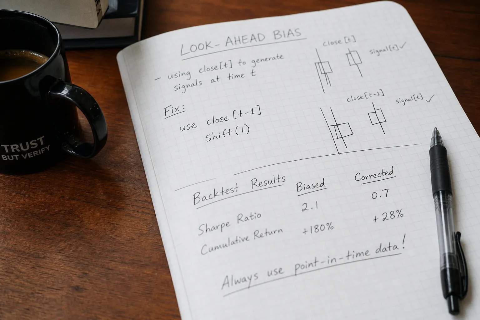
The Sharpe collapsed to 0.61. Maximum drawdown nearly tripled. Profit factor cratered below 1.2.
This is the math of how fixing look-ahead bias saved my fund — not by adding alpha, but by removing phantom alpha that was never mine to begin with. The exercise taught me something harder than any trading lesson I learned in a decade of book P&L: most of my backtested edge was an artifact of a timestamp error. The gap between a 2.4 Sharpe and a 0.61 Sharpe was a single line of code that allowed the future to leak backward into the past.
A backtest that violates point-in-time discipline is not a strategy. It is a hallucination with a Sharpe ratio.
The anatomy of a phantom alpha
Look-ahead bias is the silent killer of systematic strategies. It occurs when a model uses information that would not have existed at the moment of execution. The textbook version is stupid and obvious: using the closing price of a candle to trigger a signal that fires within that same candle, then evaluating the P&L at that same close. You buy at the close, you sell at the close, you bank the move that only existed retroactively. The Sharpe goes vertical. The trader feels invincible. The strategy dies in production within a quarter.
But the version that hit my fund was not obvious. It was a one-character bug. In my Pandas pipeline, a rolling z-score was computed using .rolling(20).mean() over a price series that had not been shifted by one bar before the signal generator read it. The signal logic looked at the current bar's moving average to decide whether to enter, but the moving average was being calculated including the current bar — a value the strategy could only legitimately observe after the bar closed. In live trading, the order would have fired on bar t, but the signal could only be properly computed at t+1. Every single backtested trade was anchored to information that had not yet arrived.
The result was an equity curve that was mechanically impossible to replicate. No co-located server, no FPGA, no fiber between exchanges would have closed that gap. The information asymmetry was not a latency problem — it was a temporal impossibility. I had built a time machine into my evaluation layer and was calling the resulting returns "edge".
What makes this particular class of bug so dangerous is that it does not feel like a bug. The code runs. The DataFrame has no NaNs where you expect numbers. The Sharpe is positive, smooth, and monotonically improving. There are no exceptions, no warnings, no obvious red flags. The only symptom is that the equity curve is too good — and if you have spent months developing a strategy, "too good" is the last thing you want to question. Confirmation bias wraps itself around the leakage and calls it insight.
| Metric | Pre-Fix (Inflated) | Post-Fix (Reality) | Delta |
|---|---|---|---|
| Sharpe Ratio | 2.41 | 0.61 | −74.7% |
| Max Drawdown | 6.2% | 18.7% | +201% |
| Profit Factor | 2.83 | 1.18 | −58.3% |
| Win Rate | 71% | 53% | −18 pp |
| Total Return (backtest window) | 38.4% | 9.1% | −76.3% |
Every line in the right column is what the strategy would have actually produced. The left column is fiction.
Identifying hidden leakage beyond .shift() errors
Most quants stop at the obvious shift error and assume they are clean. They are not. Look-ahead bias has at least six common vectors in a Python backtesting stack, and only one of them involves a misplaced .shift().
The second vector is delayed fundamental data treated as point-in-time. AAPL reports earnings on date t. The transcript, the adjusted EPS, and the revised guidance are not in your data vendor's snapshot until date t+2 at the earliest. If your signal generator reads the value at t+1, you are trading on information that no live system could have observed. This is the same family of bug as the shift error — but it hides inside a database query, not a DataFrame operation, and most code reviews miss it.
The third vector is corporate action adjustments applied retroactively. Your vendor sends you a clean adjusted close series that already accounts for the 4:1 split announced yesterday. Your backtest loads it as if that adjustment had always been present. In reality, the price on the day before the split was the unadjusted price, and any signal computed on that bar used the wrong reference point. Survivorship bias adjacent — but technically distinct. The distinction matters because survivorship bias removes names from your universe; adjustment bias warps the values of names that remain. They require different diagnostics and different fixes.
The fourth vector is index reconstitution data. When a stock is added to the S&P 500, passive flow arrives over multiple sessions starting from the announcement date, not the effective date. If your universe-construction logic reads the post-rebalance index membership at the rebalance timestamp, you have leaked between one and ten trading days of flow information into your entry price. Academic research on index additions consistently documents a price premium that begins at announcement and partially reverses after the effective date. Trading on the post-reconstitution membership list before the effective date is textbook leakage.
The fifth vector is rolling window peeking. A common implementation computes a feature on a 60-day window but evaluates the signal at the right edge of the window using the window's terminal value. That value depends on the most recent observation. If the evaluation bar is included in the window, you have leakage. The fix is structural: enforce min_periods and a strict closed='left' semantics on every rolling object.
The sixth vector, and the one I find most often in junior codebases, is vectorized signal broadcasting across the entire history before filtering. If your entry condition evaluates a vectorized expression that touches df['close'].shift(-1) — i.e., the next bar's close — anywhere in the pipeline, even in a feature that is later masked out, the computation has already contaminated the cache. Some backtesting engines preserve intermediate state that downstream filters cannot undo. The fix here is architectural: feature computation and signal evaluation must happen in separate execution contexts with no shared mutable state.
If your data layer cannot answer the question "what did I know at timestamp t?" with a strict yes, your backtest is a story, not a measurement.Point-in-time architecture: what it actually takes
Fixing this is not a one-line patch. It is a structural redesign of how data enters the system. I rebuilt my pipeline around three rules, and I would not run a strategy that violates any of them.
Rule one: every observation carries a valid_from and valid_until timestamp. Not just date. The actual moment the data became observable. For end-of-day bars, that is the market close timestamp plus any settlement-related lag you want to model. For fundamentals, it is the publication date stamped by the vendor. For corporate actions, it is the ex-date. Your signal engine only ever queries with WHERE observation_timestamp <= decision_timestamp < next_observation_timestamp.
Rule two: signals are computed against the prior bar, never the current bar. If you are evaluating at bar t, your signal must be a function of data with timestamp < t. Not ≤ t. Strictly less than. The closing price of bar t is information you do not have at the decision moment of bar t. Your code should reflect that by construction, not by convention. Convention fails. Construction does not.
Rule three: every rolling and expanding operation uses a closed='left' window with explicit min_periods. Pandas, Polars, and NumPy all support this. If your rolling window includes the current row, you have a leakage problem that will not show up in a unit test until production fails.
I also enforce a fourth rule that is not strictly about look-ahead but belongs in the same category: no usage of shift(-n) anywhere in the feature layer. A linter rule. Static analysis. If a PR introduces shift(-1), the build fails. This catches the most common junior mistake before it ever reaches the backtest. It takes ten minutes to set up and saves you months of phantom performance.
The hard part is not the code. It is the data vendor relationship. You must verify that your provider is not pre-adjusting, pre-surviving, or pre-backfilling. Many retail data feeds are "as-of reconstruction" — meaning they ship you a clean historical series that has been adjusted for splits and dividends that occurred after the bars in the series. If you trade on that series, you are trading on information that did not exist when the bars were generated. Buy a point-in-time feed or build one yourself. There is no third option that does not introduce bias.
Here is the checklist I now run on any new data vendor before a single row enters my research database:
1. Request the raw, unadjusted tick or bar archive alongside the adjusted series. Diff them. If the adjusted series has changes to bars before the adjustment event, the vendor is backfilling.
2. Audit the timestamp convention. Is the close timestamp the exchange official close, or the vendor's ingestion time? A two-minute difference on delayed feeds can introduce subtle leakage in intraday strategies.
3. Verify corporate action event dates against SEC filings or exchange announcements. If the vendor's ex-date does not match the official record, every signal computed around that event is contaminated.
4. Test survivorship handling. Request a universe snapshot from a date three years ago and compare it to the current constituent list. If delisted names are missing from the historical data, you have survivorship bias on top of any look-ahead issues.
5. Demand a schema with valid_from fields. If the vendor cannot provide point-in-time metadata, you are buying a backtesting convenience, not a research-grade dataset.
Each of these steps is tedious. None of them are optional.
Settlement cycles, execution latency, and the death of zero-latency assumptions
Even with a perfectly point-in-time data layer, your backtest is still wrong — just less wrong. Settlement cycles and execution latency are the next layer of phantom alpha.
Until very recently, US equities settled on T+2. The standard is now T+1, a shift that has materially changed the cash velocity assumptions baked into most retail backtesting frameworks. If your strategy assumes you can redeploy capital on the same bar you receive proceeds from a closing trade, your backtest is off by one to two sessions. For high-turnover systems, that gap compounds into a significant performance overstatement. The transition was mandated by the SEC and documented extensively in regulatory filings and exchange notices — understanding how settlement compression changes execution assumptions for systematic traders is not optional reading for anyone running a portfolio with daily rebalancing. The mechanics are straightforward: one fewer day of capital lockup changes your effective leverage, your margin requirements, and your reinvestment timing. If your backtest ignores these, your live P&L will underperform the simulation by a margin that grows with turnover.
The deeper issue is zero-latency execution. The default assumption in nearly every backtesting framework is that your order hits the exchange at the timestamp of the signal, fills at the signal price, and pays no slippage. This is fantasy. Real fills arrive with a delay modeled by your order routing, your venue queue position, and the market impact of your own order. A 200-microsecond delay on a fast market move can convert a profitable mean-reversion entry into a loss. A five-basis-point market impact on a size-too-large position can wipe out the theoretical edge.
What I model now, after the bias audit:
1. A minimum latency floor of 50 microseconds per order, plus a random component drawn from a fat-tailed distribution.
2. Slippage as a function of order size relative to average daily volume, using a square-root market impact model calibrated to real fills.
3. Partial fill probability when my order exceeds 1% of the bar's volume.
4. Cash reinvestment lag of T+1 to reflect the actual settlement standard.
Each of these individually shaves a small amount from the backtested Sharpe. Stacked together, they typically reduce the headline metric by 30% to 50%. That is the difference between a strategy you can scale and a strategy that exists only in your Jupyter notebook.
I want to be precise about why this matters at the fund level and not just the research level. When you raise capital against a backtested track record, you are making implicit promises about drawdown behavior, correlation to benchmarks, and liquidity terms. If the track record is inflated by 30% to 50% due to execution assumptions that no live system can replicate, your actual risk of breaching fund-level drawdown limits is dramatically higher than your models suggest. The 2022-2023 period was littered with small systematic shops that launched on backtested Sharpe ratios north of 2.0 and were liquidating within eighteen months. The common thread was not bad markets — it was bad backtests.
Rebuilding trust: from inflated metrics to statistical validity
Once the data layer is clean and the execution model is realistic, the work is not over. Look-ahead bias often coexists with overfitting and multiple testing bias. A strategy that has been curve-fit across thousands of parameter combinations — even with point-in-time data — will still fail in production if its edge does not clear statistical significance thresholds.
The minimum I require before any strategy leaves my research environment:
- Walk-forward analysis with at least four out-of-sample windows, each at least 20% the size of the in-sample period. Not a single out-of-sample split. Multiple, non-overlapping, regime-spanning windows.
- Deflated Sharpe Ratio to account for the number of strategies tested. If you tried 50 variants and the best one posted a 1.8 Sharpe, the probability that it is genuine edge is far lower than the headline number implies. The correction factor is non-trivial and grows faster than most practitioners intuit.
- Bootstrap confidence intervals on the Sharpe and the max drawdown, computed over at least 10,000 resamples. A Sharpe of 0.9 with a 95% CI of [0.4, 1.4] is not deployable. A Sharpe of 0.7 with a 95% CI of [0.6, 0.8] might be. The width of the interval, not the point estimate, is the decision variable.
- Regime tagging. Slice the backtest by volatility regime, trend regime, and liquidity regime. If the strategy only works in one bucket, that bucket's sample size is your real statistical power — not the full window. A strategy that earns its Sharpe in low-volatility trending regimes but bleeds in everything else is not a general-purpose alpha source. It is a conditional bet with limited applicability.
I also now run a purged k-fold cross-validation rather than a standard time-series split. The purge window prevents information from adjacent folds from leaking into the training set — a subtlety that most introductory machine-learning tutorials skip entirely but that matters enormously when your features are autocorrelated financial time series. The embargo period after each fold ensures that the test set does not benefit from residual label information that persists beyond the fold boundary.
The point is not to be paranoid. The point is to be honest about the difference between a real edge and a noise pattern that survived a single backtest. The market is not a casino, but it is also not a deterministic system where a backtested Sharpe is a prediction of forward returns. It is a probability matrix, and your job is to estimate the parameters of that matrix without cheating.
Look-ahead bias is not the only error in your backtest. It is the error that makes the other errors invisible.
The position
Fixing look-ahead bias did not save my fund by discovering alpha. It saved my fund by removing a metric that was lying about alpha. The 2.4 Sharpe was a bug. The 0.61 Sharpe was the strategy. The 0.61 Sharpe was not fundable at the size I had planned, and recognizing that before deploying capital is the only reason the fund is still solvent.
Every quant who skips this audit is effectively writing fiction and calling it equity research. The audit is not glamorous. It does not produce a higher headline return. It produces a lower one, and the discipline to act on what the lower number actually says. That is the entire job.
Run the structural review. Strip the leakage. Trust the smaller number. Scale only what survives both the audit and the walk-forward. Everything else is decoration on a chart that will not exist in six months.